DUGS: Data Uniquess via Gradient Similarity
Data Uniqueness via Gradient Similarity #
Summary #
This post outlines an experiment I ran to try to better understand the unique data inputs I’m using for model training. This is a modification of DVGS - “Data Valuation via Gradient Similarity”, that I’m calling DUGS (data uniquess via gradient simlarity).
Algorithm high level #
The high level idea is:
- Grab the following: a. An already trained model b. A random sampling of the data you would like to evalute of size X
- Initialize a map of
{data_point_id, uniquess_dimension}to store differing data points. - Run a training pass on each datapoint. Calculate the gradient up to a layer Z.
- Reduce the dimensionality of that vector via a random matrix
{gradient_size, uniqueness_dimension}to reduce the cost of calculating gradient similarity. (Johnson-Lindenstrauss projections) - Use cosine similarity to compare it to existing vectors in the list
- if the similarity is less than some threshold (0.3 by default) from any of the previous data points, add the new data point to the list.
Tunable parameters #
Data Set Size #
The size of the data set you are running the evaluation on will affect the runtime of the algorithm linearly.
Uniqueness dimension via Johnson-lindestrauss lemma error #
The smaller the dimension size you can reduce to, the more efficient the calculation is.
The Johnson-Lindenstrauss Lemma states that preserving the vector dimensionality within an error bound e for a dataset size N is calculated as:
k > (8 * ln(N) / e^2)
Although we are only seeking a limited number of datasets, making this match the target full dataset size ensures that there is sufficient dimensionality to understand the nuances between the dataset. The main tunable parameter is the margin of error introduced by the reduction of matrix for comparison.
For example, for 10,000 images, and a desired error of 0.001, you would have to have a base 2 dimension of roughly 8 * ln(10000) / (0.001^2)) = 73682722, or somewhere between 2^26 ~ 2^27 (rounding to some base 2 size matrix is preferred to align with scheduling on processors which primarily have cache sizes, multithreaded processor / code SM counts that align to some multiple of 2).
Number of layers to backpropagate #
This one is a model-specific choice: the more layers that backpropagation is run, the runtime complexity will multiplied by the cost to compute the backpropagation of that layer.
As a rule of thumb, I think you want to only go back to the number of a relatively low number of layers: there is an intuition that the later layers of a model are the ones more correlated to fine-tuned behavior for the specific task. This is probably the behavior that one is most interested in, such as wehn trying to find more datapoints of similar, but underrepresented data, to increase the distribution thereof.
Results #
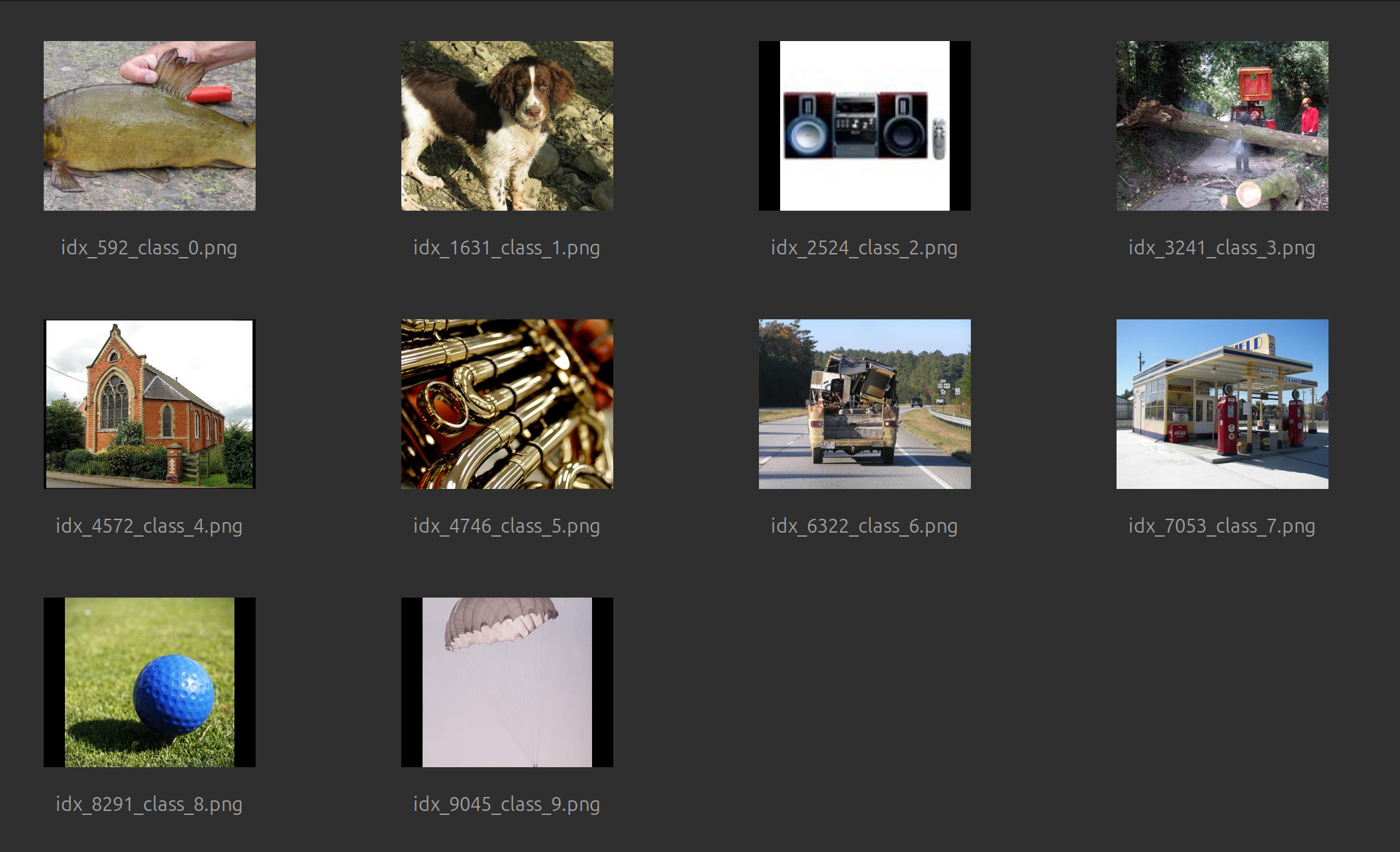
I tried this out in my sandbox against my toy model based on AlexNet, which uses the Imagenette dataset. Looking at the results visually, it looks like it was able to differentiate and find examples of each of the 10 categories:
Future Experiments to try #
- focus on the gradient of a specific layer (e.g. the embeddings)
- use dimensionality reduction via Johnson-Lindenstrauss projections
- can we use some form of k means clustering to help group the data points?
- this would be helpful to see how many “categories” of data there are.